BRICs can't hold the wall

This post first appeared at Macrobusiness

Not a day goes by when some economic commentator notes the ‘decoupling’ of economic growth of the developed and emerging economies. Europe looks almost certain to have a 2012 recession, and the US continues to have doggedly high unemployment with very soft conditions all around. Brazil, Russia, India and China, the BRICs, are meant to be taking up the slack, especially with domestic demand in China, to keep global growth on track.

But just as my suburb has a hard time decoupling from the rest of the city with which we trade our goods and services, the BRICs are nestled solidly in the layered courses of the integrated global economic masonry.

In the least reported economic news of the month, Brazil’s GDP was flat in the September quarter.  During 2010, Brazil’s economy grew 7.5%, while the year to September 2011 saw a mere 2.1% growth, with an obvious trend – down.  I am not sure what is on the horizon turn this around for Brazil, apart from a surprise boost in economic activity in Europe and the US (chart from here):

India was expected, much like China, to continue to grow at double-digit rates, but has just recorded its slowest GDP growth for two years, at 6.9%.  Particularly:

The manufacturing sector, which contributes nearly 16 percent of GDP, grew at a measly 2.7 percent, down from 7.8 percent a year ago. Agricultural output rose an annual 3.2 percent for the same period, down from5.4 percent a year ago.
The worst hit was mining, which showed a decline of 2.9 percent after growing by 8 percent in the same period last year.

Here is how Indian GDP growth has looked since 1990, with the September annual measure marked in addition to the annual measures:

The trend path for growth in India is looking to be heavily influenced by external factors.  Of course, exports make up about 20% of the Indian economy, so one must take external conditions into consideration.  Further, around 32% of the Indian economy is involved with capital investment, which can be easily scuttled should prevailing global market conditions render the financial returns unattractive.

Russia is bucking the trend a little, with GDP growth up from 3.4% annual in the second quarter, to 4.8% over the year to September 2011.  Currently this appears stable, but relatively slow.

Which brings us to China.  Well, I’m not sure what more I can add on China, but the image below shows that growth is remains high, but is doesn’t appear to be taking off in a hurry.  Annual growth has been steadily falling for the past 18 months, from 12% in early 2010, to 9.4% in the latest data:

I am not one to criticize a bit of economic stability, and the higher rates of growth on a lower base do mean that the share of economic expansion of the BRIC is relatively high.  But with these levels of growth I can’t see how the BRICs are meant to support the waning demand of the much larger western economies.  In terms ofshares of the global economy, Japan is 8.75%, US at 26%, the EU15 at 26%.  For the BRICs, Brazil is 2.4%, Russia is 1.9%, India is 2.3% and China is 7.5% – or 14.1% in total for the BRICs.

For some more perspective, the US military budget is about $1trillion pa, or half the size of the Brazilian economy, or two-thirds the size of the Russian economy.

Clearly, very strong growth rates from such a small economic base would be required to counteract even very moderate contractions in the developed world, and this is not visible in the trends we are seeing.  You can’t simply decouple the globally integrated economy while capital and goods are traded freely.

Tips, suggestions, comments and requests to rumplestatskin@gmail.com + follow me on Twitter@rumplestatskin

Economics of piracy

This post first appeared at Macrobusiness

Public debate over Internet piracy is riddled with contradictions and fingerprints of vested interests.  In the US, congress is considering the Stop Online Piracy Act (SOPA), while in Australia, an alliance of internet service providers had their proposal to crack down on piracy rejected by the Australian content Industry Group (group of music, software and games content owners).  The proposal:

…would see an ISP provide one education notice, three warning notices and one discovery notice to customers alleged to have infringed on copyright by the copyright holder, and, if a customer continued to infringe after this, the ISPs would tell the rights holder, which may then decide to apply for a subpoena to get access to the customer’s details for legal action.

Given that the application of knowledge is the engine of economic growth, one must intuitively consider copyright and patent laws as a significant burden on growth (China?).  Moves to curb piracy, as many economists are keen to point out, generally reduce consumer welfare, and in many cases reduce the profits of content owners who benefit from platform effects.

A key misapplied economic in the piracy debate is that greater incentives ‘bring about’ greater supply. That somehow, without a massive payoff, people would stop inventing and creating.  Imagine, people following their passions, even in something as obscure as blogging about economics, for their own rewards, rather than monetary payment.  History shows that creative contributions are independent of copyright and even patent protection.

Or, as The Economist magazine put it recently, “copyright theft robs artists and businesses of their livelihoods”.  Given that regulations create markets, and market actors play by the rules of the game, this point is partly true.  But is begs the question of whether markets provide better outcomes for both producers and consumers with or without copyright laws (or the evasion of the laws).

Consider the music industry.  Recent research suggests that music piracy can be beneficial to the music industry as a whole, but not those who are already superstars.

The effect of this is that piracy increases the diversity of music in the short run, and increases the supply of superstars in the longer run. In this sense, piracy is efficient, as it corrects a market imperfection.
…
This raises the possibility that opposition to file-sharing is strongest amongst those performerswhose success depends upon their fame more than their ability.

In software markets the ‘victims’ of piracy gain substantial benefits through platform effects (the result of strangely named two-sided markets).  The battle between mobile operating systems is demonstrating how platform effects work.  If Apples iOS is a platform for selling apps and music through online stores, Apple should be happy with piracy of its operating system, because the more ubiquitous their system, the more valuable their platform dependent inline retailing.  Microsoft, especially with its Office suite, shows that being ubiquitous means a cornering the market so that competitors cannot crack it.  Everyone insists on perfect compatibility with Office, because it is so common.  And it is partly so common because of the degree of piracy, rather than of sales.  Without piracy, these effects are greatly diminished.

Microsoft has even suggested that if you are going to pirate software, make sure it is theirs.

For some time, big software companies have tried to make the argument that a copy of pirated software is equivalent to a lost sale This is pretty ridiculous for a couple reasons. For one thing, there’s no reason to think that a given user of pirated software would have actually purchased a legitimate copy.
Furthermore, the argument ignores the fact that companies actually benefit in some ways from piracy, because a user of pirated software is likely to purchase software from the same maker at some point down the road. This latter point is something that even Bill Gates has admitted, even while Microsoft continues to talk tough about cracking down on piracy.
Now the company is stating more clearly that it knows there are some benefits to piracy. Jeff Raikes, head of the company’s business group, said at a recent investor conference that while the company is against piracy, if you are going to pirate software, it hopes you pirate Microsoft software. He cited the above reasoning, noting that users of pirated Microsoft software are likely to purchase from the company later on. He said the company wants to push for legal licensing, but doesn’t want to push so hard so as to destroy a valuable part of its user base.
The company recently got a stark reminder of this lesson when a school in Russia said it wouldswitch to Linux to avoid future hassles with the pirate police. Of course, this moderate stance seems at odds with the company’s recent hyper-aggressive anti-piracy push, which resulted in many mistaken piracy accusations. Either way, Raikes’ comments completely destroy the line about pirated software being equivalent to lost sales; if it actually were, Raikes would be telling people to pirate the software of Microsoft’s competitors.

Google is probably the best example of a platform business.  Their Chief Economist Hal Varian has been known to comment that whatever new software Google produces, if it increases the attraction of the Internet, then it is good for Google.

Content piracy has improved our lives, with some very minor costs to a small group of content owners whose lobbying efforts have already results in having the rules changed in their favour (thank Walt Disney). Whether this trend persists in the light of rapidly evolving content distribution methods I am not sure.

Tips, suggestions, comments and requests to rumplestatskin@gmail.com + follow me on Twitter@rumplestatskin

QLD CSG - the race for first gas

*I am now posting a daily column at Macrobusiness under the alias Rumplestatskin. This post first appeared at Macrobusiness on 18 Nov 2011.

While debate continues around land access and groundwater contamination, the coal seam gas industry in Queensland is powering ahead in a race for ‘first gas’. Which begs the question, why the rush?

It is no secret that government is a few steps behind the resource companies in terms of providing a solid regulatory framework for the industry to operate within. This is particularly the case for the management of CSG water in river catchments already plagued by their own water management issues (although DERM has released a CSG Water Management Policy and is investigating other beneficial use options).

Making substantial investments ahead of certain regulatory obligations appears a risky move on the part of the gas companies. After all, the gas will still be under your lease if you wait for some policy certainty, and sunk investments will provide substantial bargaining power to government to expand their wish-list as they finalise their policies. You won’t walk away from a billion dollar investment because the government makes you spend a little extra on over-the-top sweeteners to local communities.

The frantic pace of investment can be explained by the strategic first-mover advantages on offer to the winner of the race to produce ‘first gas’. British Gas’s Australian subsidiary QGC is a current favourite to win this race (to have their 'first gas' first), although Santos is a contender.

Stanford professors Lieberman and Montgomery published a defining article on first-mover advantage back in 1987 (ironically gaining a type of early-mover advantage on the study of first-mover advantages). They addressed the conditions under which such advantages are likely to exist, and we can use the ideas from their paper to better understand the advantages from winning the race for first gas.


Preemptive investment in plant and equipment
The first mover, or even second mover, to begin construction of pipeline and plant will gain a huge negotiating advantage during the expected consolidation of the sector; especially if the pipeline(s) is designed with surplus capacity. The owner of the first pipeline(s) can offer gas transport to other firms for less than the cost of constructing a their own pipeline. Once these first pipelines are operational, the sector will bargain a solution to avoid further uneconomical duplication, but there will be a balance of power in these negotiations to the pipeline owners.

QGC’s bargaining power was significantly enhanced by last year’s approved 15 year no-coverage declaration of its proposed pipeline from the Surat Basin to Curtis Island (see map below). This approval means that the pipeline cannot be declared for open access (which would oblige QGC to provide other gas companies access to the pipeline at a regulatory price) during this period, giving it the security to invest. QGC argued (quite rightly) that the pipeline would be economic to duplicate, and that access would not be in the public interest. But only two pipelines appear economical for the expected production of the area, so there will be second mover advantages as well.

But QGC’s no-coverage declaration also added significant extra time pressures, since the approval will lapse after three years if the pipeline is not constructed and in use. Santos noted in its submission to the National Competition Council in April 2010 that QGC is unlikely to meet that three year deadline, and hence their pipeline may not be protected from a regulatory access regime. The pressure is on for QGC:

Consolidation of the sector is also likely to occur in other parts of the production chain (see below), including upstream exploration and drilling, and in particular the liquefaction stage on Curtis Island where the industry is likely to negotiate a more efficient option than the four separate plants:





Overall, the sector may consolidate extraction rights themselves by a number of means. The first mover (to construct a pipeline and plant) may buy out other tenements from a strong bargaining position, or perhaps partnerships and joint ventures will emerge with other gas producers, or even straightforward private arrangements for utilising the first mover’s pipeline and plant.


If QGC and Santos build pipelines and plant with excess capacity, they can take a share of rents from other gas companies through these types of consolidations, which is publicly their intention:

“BG Group now has the strategic advantage of being the first to make a financial decision, with construction of its project to begin immediately.
Consolidation in the CSG and LNG sector in Queensland is widely expected, and as the “first mover”, BG will be one of the main players with whom other hopefuls will now want to talk.” (here)

Given this likely eventuality, other players have pushed through with plans of their own to stay in the race for the top two, given the payoff for success is so great:

The $35 billion Australia Pacific LNG (APLNG) joint venture will theoretically become neighbours with BG, Santos/Petronas and Shell, which have all announced plans to build separate plants on Curtis Island, off Gladstone, in Queensland.However, consolidation is expected in the sector.

Switching costs and buyer choice under uncertaintyFinally, the leaders of the race for first gas will have greater opportunity to monopolise contract negotiations, and develop strong buyer relationships. The typically long contracts in the gas market reinforce the dominant position of first movers. Santos, for example, currently has a 20 year contract with Petronas, while QGC has a 20 year contract to supply CNOOC, a Chinese state-controlled oil producer.

As a final note, the pace of development is important financially simply by bringing forward returns on a multi-billion dollar investment.

So how do you get a first-mover advantage? Lieberman and Montgomery suggest the following:

A firm gains first-mover opportunities through some combination of proficiency and luck. Various types of proficiency may be involved, including technological foresight, perceptive market research, or skillful product or process development.

I would add strong relationships with government officials, which can help push through approvals ahead of the pack, and often ahead of the formation of government policy.

This regulatory relationship is clearly a real concern. Santos has cautioned against regulatory interference in the expected industry consolidation process, through, for example, unpredictable outcomes of no-coverage applications, given the massive impact it will have on bargaining power between gas companies. Favourable treatment in such deliberations is a true source of industry power.

I am not a gas industry insider and there may very well be some subtle considerations I have overlooked. But on the surface, the evidence is strong that the pace of development, beyond the pace of development of environmental regulation for CSG production, is being primarily driven by the race for first gas.

This means there is a trade-off between the pace of development, and the quality of the development these environmental regulations. A slower pace of development may provide incentives to better optimise investment for the industry as a whole (rather than the first mover), and opportunities for the communities affected by the industry’s development to better understand what is happening before having their input into policy making.

This leads to another question, would eliminating advantages to the first-mover slow development to allow regulation to catch up?

This is not as simple as it might sound. The threat of open access declarations could have the exact reverse effect of completely rendering the pipeline unviable. Of course, government could simply build one and charge a fixed rate of return charge to all gas companies. I wouldn’t, however, expect the operation of this pipeline to be particularly efficient, and it would still lead to lobbying by the industry players over the operation of the government’s access regime.

A creative solution might be to regulate against exporting LNG from Curtis Island until a date sufficiently late for all companies to be contenders for completing their proposed pipeline and plant. Perhaps this will encourage consolidation of the sector prior to gas being delivered. But in all honesty, I can’t think of a way to eliminate the race, without eliminating some of the benefits of CSG development, and without picking winners.

Maybe the simple solution is for government to take a hard line when it matters, such as during assessment of environmental impact statements, and incur some delays at that point for the sake of nudging trade-offs in favour of the wider community. Delaying approvals at early stages may have provided the time to collect better data about the geology and underground hydrological effects of CSG extraction.

I personally believe CSG development can be a great benefit to Queensland and Australia over the next quarter of a century, but the political class being targeted by industry lobbying needs to be aware that their hard hat photo opportunities and premature approvals are inherently trading off benefits between external stakeholders and late entrants, and the industry’s first mover(s).

US observations

Two observations today.  The first is the graph below showing the median houshold income in the US since 2000 (ht.Felix Salmon).  Suprisingly the recovery from the 2008/09 recession has not resulted in an income boost, but in fact a dramatic continuation of the decline.

The second observation is that big banks on Wall Street are participating in a program to 'buy' their own police (ht.Yves Smith).  Which is all the more ironic this week as the Occupy Wall Street protestors rally against regulatory capture and the greed of the corporate world in seeking pursuing these ventures.  These officers are paid a token hourly rate by participating corporates, but their training and insurance is provided by the city.  Privatise profits, socialise losses.  That's not capitalism.

The fall out from the financial crisis is not over.

Media watch – cosleeping report

Within 24 hours of the Victorian Coroner’s Prevention Unit releasing a background report into infant deaths from co-sleeping (parents sharing beds with infants), no less than 31 media outlets have reproduced the media release beneath fear-inducing, but unrelated, headlines.

• Babies sleeping with adults at greater risk of death: study
• Landmark study reveals dangers of sharing bed with babies
• Fear as babies die in their sleep
• Cuddling Leading to Infant Deaths in Victoria Triggers Investigation
• Sharing Bed Could Lead To Death of Baby?

A credible journalist would have read the Coroner’s background study and found that its conclusions are nothing like what the headlines suggest (perhaps the subeditors need to pull their heads in). As the study itself notes -

The study was restricted to a case series of deaths, for which no comparison groups were available. Without being able to compare the proportion of co-sleeping among the fatal cases to the proportion of co-sleeping among non-fatal cases, it is not possible to provide an estimate of the increased risk of death attributable to co-sleeping.

In fact, the study is just an analysis of a selection of case-study data to inform an ongoing investigation, for which the Victorian Coroner is currently seeking input.  The investigation was triggered because the proportion of unexplained infant ‘sleep’ deaths associated with co-sleeping increased from 21 to 45% between 2008 and 2010 (7 deaths to 15 deaths).

Is it too much to ask that journalists actually read the source of their article before writing and offer an objective view, rather than induce fear in new mothers with unrelated headlines and loose presentation of the facts?

If any of these journalists had modicum of mathematical aptitude they would have realised that proportion of infant deaths from co-sleeping is meaningless without knowing the proportion of infants who co-sleep.  If 90% of infants co-sleep, but the only make up 45% of unexplained sleeping deaths, then that is some evidence to show it is probably not a factor.

And most bizarrely, if the rate of co-sleeping is constant, than some other factor MUST be to blame for the changing ratio (even if that factor is random variability).

Unfortunately the evidence on sleeping habits of infants during this period is limited.  This survey from 2008 shows that, in a sample of 6383 breastfeeding mothers with babies under 1 year old, about 37% of mothers co-sleep with their baby. If that ratio has increased since that time it may very well explain most of the data seen by the Coroner.  Other evidence suggests that breastfeeding mothers are three-times more likely to bed-share, and the ABS estimates that about 48% of babies under one year of age are breastfed (consistent between 1995 and 2001), although the proportion declines from about 85% to 30% over the period.  This gives a rough picture of co-sleeping habits in 2008 of about 29% - with co-sleeping deaths at 21% in this period.

Given the massive limitations of Coroner’s report, and the inherent variability in the year-to-year infant deaths statistics (the same debate occurs around pool fencing laws), the report itself seemed rather lacking with regard to the extensive existing literature on the topic.  For example, this research surveyed 4656 families internationally about sleeping arrangements and found that

Rates of bedsharing varied considerably (2–88%) and it appeared to be more common in the samples with a lower awareness of SIDS, but not necessarily a high SIDS rate.

A summary of the results is graphed below.

One major factor limiting the understanding of infant sleep death risks are omitted variables.  The ABS surveys on breastfeeding show strong trends between mother’s age and educational attainment and breastfeeding habit.  Also, the confounding factors of alcohol intake and smoking (and other health risk exposure) of the infant need to be taken into account to begin to point the finger at sleeping arrangements.  With this data available one can separate the impact of co-sleeping risks from the impact from other health risk on infant ‘sleep’ deaths. No doubt and the Coroner’s inquiry progresses these issues will be addressed in detail.

The creative destruction of retail

The great Australian retail adjustment is happening now at a store near you.

• Myer Managing Director Bernie Brookes recently announced the retailer’s plans for more serious efforts in online retailing, with $9million set aside to improve Myer’s online presence.
• Target yesterday sent a letter to suppliers explaining why they are going to pay 5% less for all their goods from now on – take it or leave it (ht: Adrian).
• Mark McInnes, head of Premier Investments, the owner of Dotti, Just Jeans, Portmans and Jay Jays outlets, has closed 19 stores and threatens to close more if he cannot bargain down the rents paid by his remaining stores.
• Masters, the hardware joint venture between Woolworths and Lowe’s Companies Inc, opened its first stores early this month to compete with Bunnings in the hardware and homewares market.
• Dick Smith has also had his say about the supermarket discounting wars and executive pay.

Not only are the retailers making some tough decisions, but shopping centre owner Stockland, whose CEO Matthew back in February noted the sunny outlook for their three Rs strategy – residential, retail and retirement – is finally coming to grips with reality and is rushing to offload a selection of retail property holdings.

Read full post at MacroBusiness...

How the CPI hid the housing bubble

Recent discussions about the CPI have brushed over a key change that occurred in the construction of the index in 1998. In its 13th Series the CPI became a pure price index utilising an acquisitions approach, rather than a cost-of-living index utilising an outlays approach. One feature of this change is that it removed land costs for owner-occupiers – something which doesn’t appear to reflect reality and provides some intriguing results.

The move to an acquisitions approach was in line with the broader philosophy of inflation measurement at the time. The OECD noted this philosophical change, commenting that modern inflation indexes:

…have been constructed with the aim of measuring monetary inflation rather than measuring the broader concept of the cost-of-living, which has a more welfare-oriented philosophy.

The ability to judge economic conditions with any degree of confidence is best achieved with both a cost-of-living index and a pure price index. Since 2003 the ABS has published its Analytical Living Cost Indexes for households (ALCI) to play the role of a cost-of-living index. This measure uses the outlays approach, and one would expect it could reveal some of the costs associated with the land price boom of the early 2000s.

Yet the ACLI for employees is within 3% of the CPI after thirteen years. I can reconcile this outcome fairly closely with my own calculations using their method, and estimate a cost-of-living index around 0.3 percentage points higher than the CPI, on average, over the past 13 years. You will notice how this index tracks the CPI prior to 1998 (this method actually was the CPI calculation at that time). The graph is below.

However it is a little strange that the ABS conducted an evaluation of the impact of different treatments for housing in the CPI back in 2006 and found that a full cost-of-use approach, with weighting consistent with HES data (which the CPI does not have), would have produced a CPI between 1998 and 2003 more than double the official number (for Sydney). Considering that the official ALCIs were slightly lower than the CPI over this period, it is an odd situation indeed.

The reason for the discrepancy can be traced to a gap in the mortgage interest charge index between 1998, when it was removed from the CPI, and 2003 when it was added as a separate item in the ALCIs. The ABS cannot provide the data to bridge this series gap and has suggested that simple interpolation is inappropriate due to rebasing of the ACLIs during this time.

Below is a graph of the mortgage cost index rebased as per the ABS explanation and interpolated using the data on mortgage interest paid as a proportion of household income from the RBA. This mortgage interest charge index can be compared to the ABS house price index (HPI) from 1994. We can see that from 1998-2003 the HPI increased 64% while the mortgage interest charge index increased just 24%. Yet the mortgage rate was the same at the beginning and end of the period. We also know that the HPI was originally developed as an input to the mortgage interest charge index. It is this data which gives a cost-of-living estimate matching the published ACLIs.

But it a more realistic reconciliation of the mortgage interest charge index would have this index tracking the HPI during the 1998-2003 period as shown in the graph below.

Using this data the cost-of-living index is about 0.5 percentage points higher on average since 1998.

So what led to the current mysterious situation surrounding housing treatment in cost-of-living indexes, and the complete removal of land from the CPI?

In 1997 the RBA argued strongly to remove the price of land from the CPI in its submission to the 13th Series CPI review. The RBA argued that including a mortgage interest component in the CPI would result in an inflation measure that is amplified by monetary policy responses to inflation itself. They say 

At a time when inflationary pressures are increasing, interest rates are being increased to combat those pressures. The interest components of the CPI also rise, adding a short-term impulse to inflation as measured by the headline (or total) CPI.

That is a reasonable argument in my mind. But their logic for me breaks down a little when they say that “the acquisition of a house is really an investment activity, rather than consumption”.

So why include it at all? Why not use an imputed rent for owner-occupiers to be consistent? Or use mortgage interest as a proxy for the annual benefits flowing from owner-occupied housing? Simply excluding land purchase costs without any proxy for the annual use of land is totally inconsistent.

To me, you need to choose one treatment or the other. Either add the full cost of homeownership as a lump sum, either in the form of house prices or adding the cost as a periodic payment by the home-owning household to itself in the form of imputed rents. The RBA canvasses this approach in its submission but noted that this may cause a ‘disproportionately large’ weight to the housing basket.

The weight to be assigned to the Housing group would need to be adjusted to recognise that all owner-occupier households are paying ‘imputed’ rents to themselves, resulting in a disproportionately large weight on housing in the CPI.

The RBA submission mentions a number of times that they see a high weight on housing in the CPI basket as unfavourable. For example, they note that by excluding the land component of house purchases the weight on housing would be substantially reduced. By international standards, our basket weight to housing is low at 16.43%. Germany has a 20.33% weighting for rents alone (and another 1.4% for home maintenance), the US has 30% allocated to rents and owner-occupied imputed rents, the UK has housing at 20.9% and the Netherlands at 23%.

This is all very odd since the weighting of housing in the CPI is a key determinant of the CPI itself. The ABS noted this issue in their 2006 analysis, showing that the full weight of household expenditure on owner-occupier user costs was around 15.8% in 2003, yet the CPI measure allocated just 7.1% to owner-occupied housing costs.

Most interesting of all is that the RBA concludes in their submission that “excluding interest charges would in no way distort the outcome over the long run”. Well, I’m not sure just how long the long run was in the minds of the RBA staff at the time, but they probably weren’t thinking about periods longer than a decade. The mortgage interest charge line in the third graph above may very well return to the level of the current house purchase cost line. But as you can see, for this RBA assertion to hold true, home prices or interest rates need to fall quite a way.

Quality adjustments to the rent price index are another strange feature of the treatment of housing in CPI. The scope of quality adjustments to the rental price index has led to this absurd result.

…that for the period December 1994 to December 2005 the average rent paid by private tenants included in the ABS Survey of Income and Housing increased by 41.1%, while the increase in the CPI rental component was 22.9%

As I said last week, it is about time that the silent quality adjustments creeping into the CPI be made public so we can better evaluate just what this means out there in real life.

For some reason the RBA doesn’t seem too bothered by changes in the CPI methodology, particularly relating to the price of housing.

Currently, housing-related costs – including rents, utilities and the cost of building new dwellings – account for around 20 per cent of the CPI, the largest share of any single group. Broadly speaking, the housing component of the CPI shows the same general pattern as that in underlying inflation, although the recent moderation is less pronounced.

The bank also has a particularly strange argument to explain why high house price inflation is not a concern. They state that “the large run-up in Australian house prices that was driven by the adjustment to low inflation ended in late 2003.” Yet inflation in the 1990s was around 2.1% on average and increased quite dramatically from 1998 to 2003 during the run-up in house prices. Of course, the RBA doesn’t use headline inflation measures anyway. They have their own favourite price measure – the average of the weighted median and trimmed-mean CPI.

So where does that leave us? We can combine the main areas where housing has been stricken from the CPI—the removal of mortgage costs, quality adjustments to rent, and reduction in weight to homeownership costs—to see what difference it would make had the pre-1998 methodology been continued. The resulting MacroStats cost-of-living index is plotted below against the headline CPI.

This measure uses a continuous weighting adjustment between weight revision years (1998, 2000, and 2005), and applies a weight to owner-occupied housing costs consistent with the weighting in the ABS 2006 publication on housing in the CPI as well as applying the amended mortgage cost index in lieu of the new house purchase index. It also makes a slight adjustment to the rent price index since 1990 (20% increase in growth rate compared to the almost 100% increase observed using mean measures) to remove a little of the quality adjustment.

We can again see how this measure tracks the official CPI very closely until 1998. Since 1998 it is 0.73 percentage points higher on average (or 3.8%), and in the period 2001-2008, it averaged 1.3 percentage points higher (or 4.4%pa). That gives you some idea of how significant the 1998 methodological shift in the CPI was in disguising housing inflation and creating a feedback loop with lower monetary policy.

So what does this all mean? For me, there are four key lessons.

1. The treatment of housing needs to be consistent in a pure price index with its treatment of a flow of services. You can’t include a capital cost in the form of new house purchases without including land, but also include a cost-of-service price for rental homes. My recommendation is to treat owner-occupied housing in the form of imputed rents with a weight in the basket approximating the weight to mortgage payments.
2. If homeownership is a policy goal, cost of living indexes should treat home buying and renting households separately. This will ensure that any policy aimed at making homeowning more attractive can be evaluated by comparing these metrics.
3. In all both pure price and cost-of-living indexes quality adjustments, particularly regarding heavily weighted items such as rent, need thorough explanation and should be published alongside standardised measures such as mean and median prices.
4. Be extremely careful comparing economic performance between time periods using the CPI to deflate nominal price to real prices.

Quarry Australia has no people

Fungibility is a feature of a good where two items of that good are so close in their features that they equal substitutes.  Currency is the ultimate example.  If I lend someone $50 it doesn’t matter to me whether that same $50 note is returned, or another equally good $50 note.  Other fungible goods include standardised commodities like wheat, raw metals, oil.

But is labour the same?

I doubt many businesses would be happy to lend an employee for a few days work elsewhere then receive a different person back when the job is done.  While there are people with very similar skills and experience who may be suitable substitutes, this is not the case in general.  The idea that some workers are subsitutes for some others, but all workers are not substitutable, forms the great divide between the policy prescriptions of the Austrian economists and the Keynesians, and may be one reason for the apparent failure of Keynesian stimulus to ‘create’ jobs in the US.  It also explains why labour costs in some industries can rise even with relatively high unemployment.
...
Read the full article at MacroBusiness.

Stimulus for a recession that never was

*I am now posting as a regular contributor at Macrobusiness under the alias Rumplestatskin.  I will be posting copies of posts at both websites for the coming weeks.

 

Hands up who knew that Australia avoided a technical recession in the aftermath of the GFC? Kevin Rudd certainly got some miles out of it, noting in his farewell speech how proud he was of that fact and the role his government played.  But as usual all is not what it seems.  The Keynesians shouldn’t be celebrating just yet, as Professor Tony Makin explains:

In the aftermath of the GFC in September 2008, Australia’s nominal GDP, real GDP measured on an income basis and on a production basis, as well as real GDP per person, all fell over two successive quarters, as did various other national income measures that account for the slump in export commodity prices (or terms of trade) at the time.

Of the many national accounts series the Australian Bureau of Statistics publish, the only one indicating there wasn’t a recession was the real, or price level adjusted, national expenditure series.

In the US, a recession dating committee of the National Bureau of Economic Research uses a battery of macro-economic measures, not just the somewhat arbitrary two successive quarters of negative real GDP.

If the behaviour of Australia’s business cycle in the aftermath of the GFC had been assessed by an independent committee of economists with reference to a broader range of macroeconomic indicators in this way, a recession, albeit mild, would most likely have been declared for 2008-09.

In his more technical analysis of the impact of fiscal stimulus, Professor Makin kindly summarises some of the other key measures in the National Accounts (in the below table), and notes the following:

Though routinely ignored in economic commentary, the real gross and net domestic and national income series are especially important measures of Australia’s international macroeconomic performance because they reflect the impact of the terms of trade (or ratio of prices received for exports to prices paid for imports) on the economy.Other notable recession features included declining total hours worked (for 5 straight quarters in the market sector), falling compensation to employees and increased unemployment.

But what is most interesting from the good professor’s analysis is the delay he observes between the recession and the appearance of fiscal stimulus in the data.  He finds that:

Federal public investment actually contributed negatively to total expenditure over the critical December 2008 and March 2009 quarters, being -0.2 and -0.1 respectively, as did public investment by State and Local governments. As a result of administrative delays in implementing infrastructure spending, total public spending did increase by the end of 2009, but only after the worst of the GFC had passed, and then arguably crowded out private investment spending at the time.

Now there are obviously administrative delays to get $40billion spent on school halls and home insulation (not so much with cash handouts), but this very practical aspect of such Keynesian intervention must be addressed – how can governments time economic stimulus measures appropriately unless they have perfect foresight?

Professor Makin argues that the drop in the value of the Aussie dollar, and interest rate adjustments, are what ‘saved’ us from a technical recession, and not the delayed fiscal spending. Not only that, but government spending ramped up just as the private sector was itself recovering from the downturn, arguably crowding out private investment (although I personally wouldn’t suggest this is a major factor).

While no doubt Australia’s economic performance of the past two years has been exceptional by any global measure, our combined monetary, exchange rate and fiscal stimulus, with their various time lags, were also exceptional over this period and arguably excessive.  Now that these measures have run their course perhaps our economy will have a second chance to adjust to a more stable level, with higher savings and lower spending.  Today’s National Accounts numbers will provide further insights into key sectors of the economy now that the fiscal stimulus measures have fully ceased.

The Rolex economy

*I am now posting as a regular contributor at Macrobusiness under the alias Rumplestatskin.  I will be posting copies of posts at both websites for the coming weeks.

I was recently in touch with a Swiss friend of mine who casually mentioned that the Swiss government was taken action to help their economy adjust to the undesirable strength of the Franc (CHF), shown in the charts below.  Given that the Australian government and the RBA have been silent about the disruptive impact of the high dollar on manufacturing, tourism and education, it makes for an interesting comparison.

On the financial battleground, it appears that not only has the Swiss government lowered interest rates to zero and intervened to increase liquidity and help weaken the currency, they are also talking about deposit fees to make their currency less attractive to the tsunami of financial speculation surging around the globe.

(Also bizarre is that this high currency nation perched in the Alps has a GDP which is comprised of 50% exports, with net exports at 12% of GDP.  Indeed Switzerland has been a net exporter of goods and services every quarter since 1981.  Meanwhile our exports are just 21% of GDP and we have been a net importer in annual terms for decades.)

In addition to directly targeting the currency, the Swiss are taking on the challenge by trying to boost productivity to ‘make room’ for a higher currency.  The Swiss Commission for Technology and Innovation (CTI) has boosted efforts to commercialise new technologies to offset currency impacts on Swiss manufacturers by doubling the value of grants accessible in the next twelve months, and broadening the qualifying criteria. After all, innovation in production techniques is the key to improving productivity and economic growth.

No doubt such investment is driven by Johann Schneider-Ammann, Head of the Federal Department of Economic Affairs, who appears to understand and promote the role of productivity as the driver of growth.  In a recent speech entitled Strengthening Switzerland as a manufacturing location, made at the opening of a new Nestle production centre, he made the following comments (my emphasis).

• We must continue to invest in training, research and innovation. It is essential for personnel at all levels to be well trained. Thanks to our dual-track system of vocational and professional education and training, we have programmes with a strong practical focus. Education, research and innovation must be given top priority. Switzerland should continue to produce talent of the highest calibre. Only in this way can we maintain our leading innovative position and continue to be competitive.
• Market liberalisation and the removal of trade barriers are essential for Switzerland, and especially for a multinational company such as Nestlé. We are familiar with the problems and challenges which the global product trade faces on a daily basis. I therefore aim to ensure that we have access to the important growth markets and remove unnecessary trade barriers within Switzerland and abroad. I am in favour of extending our network of preferential agreements with major dynamic economies such as China, India and Russia.
• I am aware of the agricultural policy framework under which food companies such as Nestlé produce in Switzerland. These are currently compounded by the strong Swiss franc. This is weakening our export competitiveness considerably. I assure you that I will do everything I can to maintain or improve current conditions for Swiss companies which export abroad including the food industry.
• The labour market in Switzerland is flexible, and should remain so. The freedom of movement between Switzerland and the EU is to our overall economic advantage. Nonetheless, we still require accompanying measures to ensure that this advantage is not weakened. I also believe in the importance of nurturing a healthy relationship between social partners.

One could argue that if Australia did not have mineral and energy wealth to fall back on, we would be doing similar things and would have our leaders making similar speeches out of necessity.  Perhaps that’s true.  But choosing the short term lazy option of quarry Australia, which has been promoted by the RBA and others, is not a recipe for a stable and prosperous economy.  As I have said before:

My main concern is that frighteningly, the RBA, and probably much of the government, sees Australia’s future as a single bet on mining, and is willing to sacrifice much of the remaining economy for this to happen. Unfortunately this is a lose-lose proposition for most of the country.

All other sectors of the economy lose while the mining investment booms. When it crashes, we all lose because there is nothing else left in the economy to absorb capacity in a relatively short period. Remember, the minerals will be in the ground if we don’t mine them now, but the decades of production chains elsewhere in the economy are easily destroyed and slow to rebuild.

I acknowledge that the RBA has a single tool in its toolbox, but surely the message we should be hearing is that a strong and stable economy is a diverse economy. Quarry Australia is a very volatile and risky place to want to be.

We could learn some lessons from Swiss economic policy.

Improving the house price and income debate

While the RBA has warned of the risks of leveraging into the housing market on national television, they, and other analysts, have also presented a stable picture of the housing market, by estimating a house price to household income ratio of about 4x, and accompanying such analysis with statements like the ratio of housing prices to income has been reasonably flat for a number of years. 

Or, when he is at his best, Glenn Stevens can calm the nerves of recent home buyers with comments like this -

The other thing I’ll say is that it’s quite often quoted very high ratios of price to income for Australia, but if you get the broadest measures, a country-wide price and a country-wide measure of income, the ratio it about 4 ½ and it hasn’t moved much either way for 10 years.

I think I can safely say that most of Australia would disagree with this assessment of stability in the housing market or support from economic 'fundamentals'. Indeed even the RBA's own representations seem a little schizophrenic on the subject, with a recent report noting that the price-to-income ratio actually increased by 50% between 2001 and 2004.

Dwelling price growth significantly outpaced growth in household disposable income, with the nationwide dwelling price-to-income ratio rising from around 2½ in the mid 1990s to a little over 3 by 2001 and then to 4½ at its peak in early 2004.

Which is it Glenn? Did the ratio increase by 50% in that period, or hasn't it moved much either way for ten years?

One reason for the clash between public views on housing and the 'stability stance' we see out of the RBA is that the RBA grossly overestimates household incomes.

I have examined the data used by the RBA and other analysts from the National Accounts (Table 14), and tried to replicate their method and reconcile the differences with ABS household survey data, which more accurately reflects household income available for current consumption. It is possible, and I have shown my results in shown in the table below.

ABS household survey data shows that at the beginning of 2010, the average household income was $88,113 before tax and $74,360 after tax. This closely reconciles with my own household income estimates from the National Accounts data in 2010 (within 1.3%). Unfortunately due to the need to estimate the total number of households between census years, this method has quite a large margin for error.

Given the average national dwelling price at that time was $447,994 and the median about $415,000, we are definitely in an uncomfortable range of price-to-income ratios, with 5.0x in average terms using before tax income data, and around 6.0x in after tax terms. In terms of median incomes and dwelling prices, the ratio is probably closer to 5.6x before tax, and 6.8x in after tax income (as recently estimated by fellow blogger Leith van Onselen).

This happens to match the data produced by Rismark (here), after they revised their average price-to-income ratio up after noting the discrepancies in the unadjusted National Accounts data.

While I don’t believe household income and house price comparisons are the best indicator of the state of the housing market (preferring comparisons of rents to incomes and yields to other rates of return in the economy), it does seem that we can use the national accounts data to give a decent regular estimate of household incomes for those who wish to use them for analysis.  Maybe the RBA should try it sometime.

Also important to note when comparing incomes to prices is that the debt service ratio, measured as interest payment against incomes, can be misleading.  Since this measure is also published by the RBA, I assume they rely upon it in some way. 

Below is the household finances graph from the RBA chart pack (available here). We can see that, following the declines in interest rates at the end of 2008, household interest payments have settled at around 12% of disposable income. Note again that the RBA disposable income measure is probably overestimated (there is no specific note about the treatment of imputed rents), meaning the both measures are probably underestimated. But in any case the trends over time still hold.

What we need to consider here is that the interest paid graph shows what might be called a 'debt-service' ratio (although not in the true sense which would cover principle repayments). In regard to the surging household debt the RBA notes that the ...structural decline in interest rates has facilitated the increase in household debt ratios because it reduced debt-servicing costs.

That is true, but would only explain an increase in debt that accompanied flat interest payments as a proportion of income, not increasing interest payments (as I have explain in detail here).

What is also overlooked is that at lower interest rates the difference between the payment of just the interest on debt, and the repayment of interest and principle (to actually reduce the loan balance over a fixed period), greatly increases. For the same interest payment, a high debt balance with a low interest rate is more difficult to repay than a low debt balance with a high interest rate.

The table below shows the amount of debt that a household with an income of $75,000 could service with 20% of their income ($15,000pa) at different interest rates. While a halving of interest rates means the household could double the loan amount and pay the same interest payment, the loan they could actually repay over 30 years increases by far less (as shown in the right hand column).

It is also important to understand this relationship when comparing our household debt burden internationally. The RBA usually makes such comparisons without noting the importance that interest rates make to the burden of this debt on households. Given that mortgage rates vary between 7.5% in Australia to 2.5% in Switzerland and 3% in Germany and much of the EU (and noting the tax deductibility of mortgage interest in Netherlands), these differences are important. 

I will finish this analysis by presenting three graphs. 

First is a graph of the household occupancy rate. The reason to include this is that while household incomes may be still growing nicely, the number of people per dwelling has been increasing since late 2005, so in per capita terms incomes are not looking as good.

The second graph shows the contributions of insurance premiums and claims to household income (which I removed in my income estimation method). When this number is positive it means that household insurance claims were more that the premiums paid in that period. That’s why we see a massive spike in February 2011 from the claims relating to floods and cyclone Yasi (and amongst other things, the Black Saturday Bushfires in early 2009 – note the data is very cyclical with a summer peak). It seems odd to have either the insurance premiums or claims in estimates of household income (although makes up just a fraction of a percent of the total).

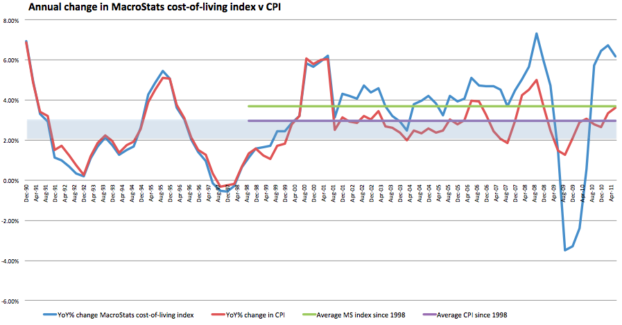
The third and final graph compares the growth in household incomes using each method with the ABS capital city price index. Of course, I have chosen an arbitrary baseline at June 2001, but I do note that mortgage interest rates then were the same then as they are now (indeed mortgage rates were about the same as now back in 1997 - see here), so the deviation observed could easily be interpreted as an overvaluation of housing.

What the graph mostly tells us is that there is a pretty solid reason so many people believe that house prices are historically high and are more likely to fall than rise in the near future, being supported only be our willingness to incur debt, and not our incomes.